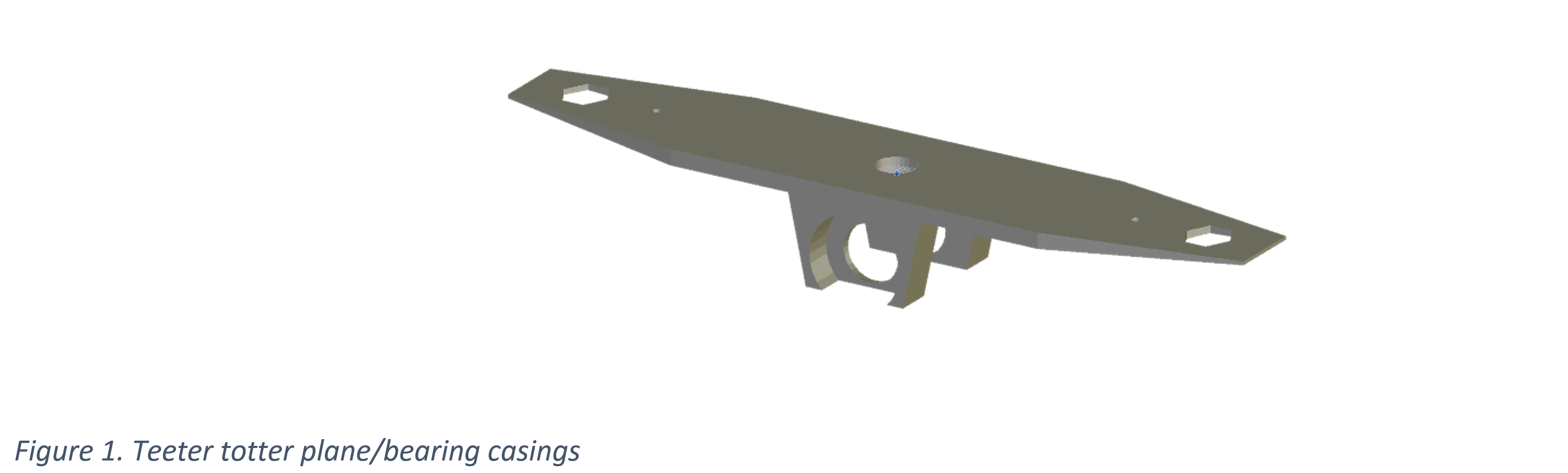
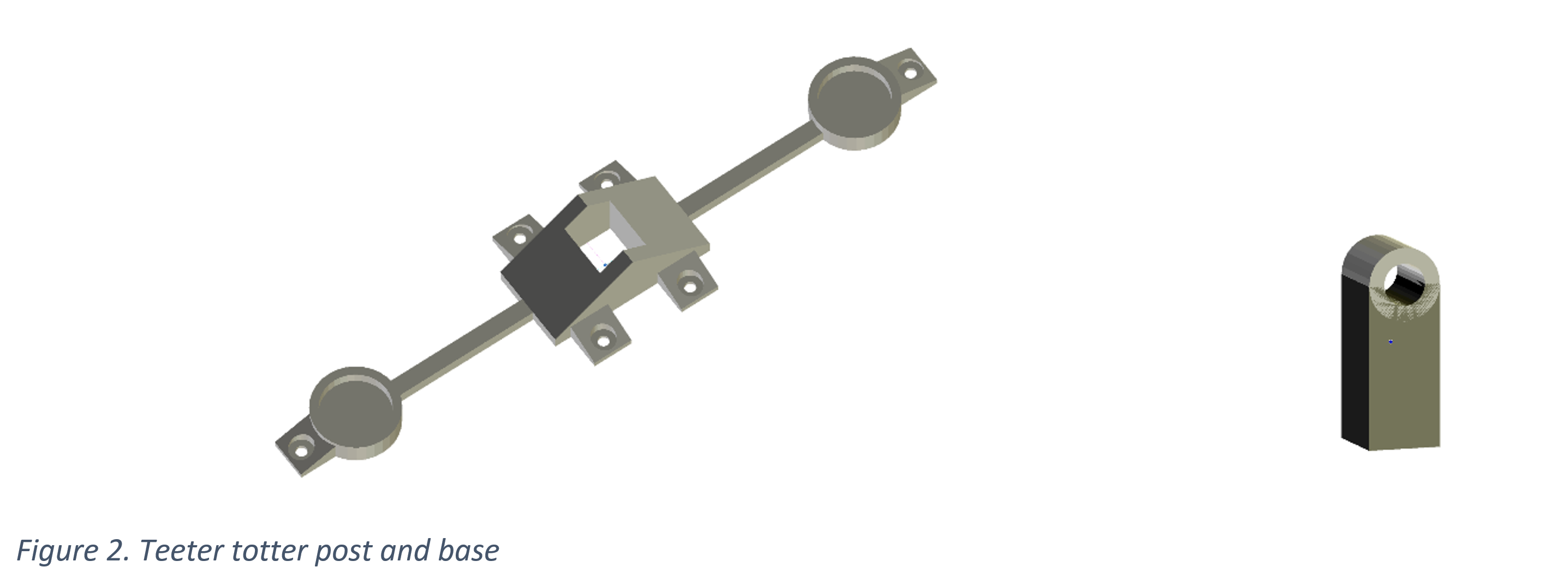
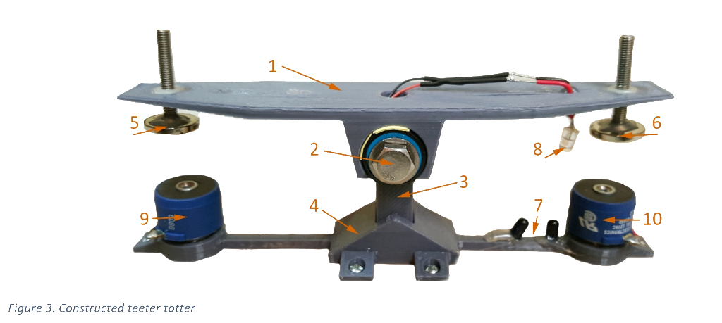
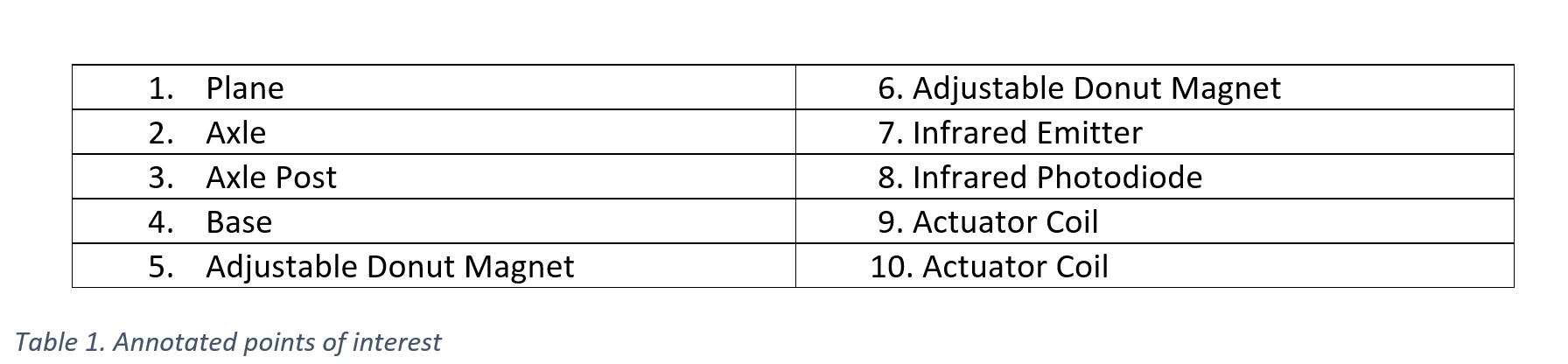
This is part two of a two part series… check out the construction and characterization of the teeter-totter in part one!

Buy me a coffee!

First things first, here are some results. These two GIFs show how a phase lead compensator can significantly improve a system’s ability to recover from outside disturbances. Keep scrolling down if you’re interested in how this was implemented!

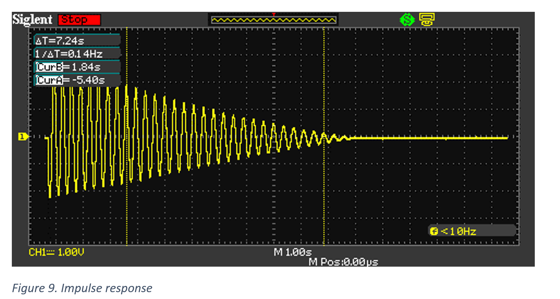
Uncompensated impulse response:

Compensated impulse response:

Abstract – Previously, a teeter-totter was constructed and modeled in the continuous time domain. This model will be brought into the z-domain so that it can be controlled by a sampled data discrete time control system. A NI Data Acquisition Tool as well as an ARM Cortex-M4 will be used to implement the control schemes.

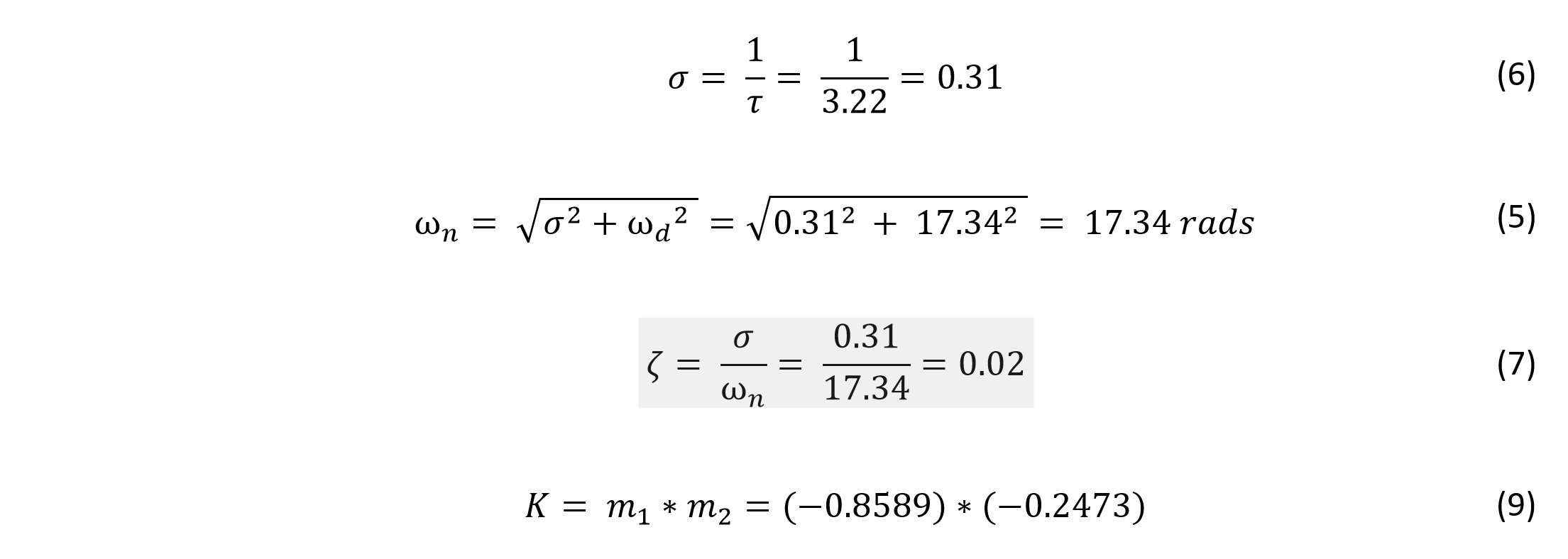
The first control system to be implemented is the open loop controller, allowing the system to reach a reference point with minimal overshoot and settling time, but still remaining vulnerable to disturbances.

To reject disturbances, a closed loop lead compensator will be implemented, allowing for rejection of disturbances, but contributing notable steady state error.

To get the best of both worlds, the lead compensator will be combined with the open loop controller to create a “Bridged-T” network. This will allow for low steady state error due to the open loop controller and rejection to disturbances due to the lead compensator. This control system will be implemented on an ARM Cortex M4 microprocessor rather than the NI-Data Acquisition tool used for the phase lead compensator.

The z-domain

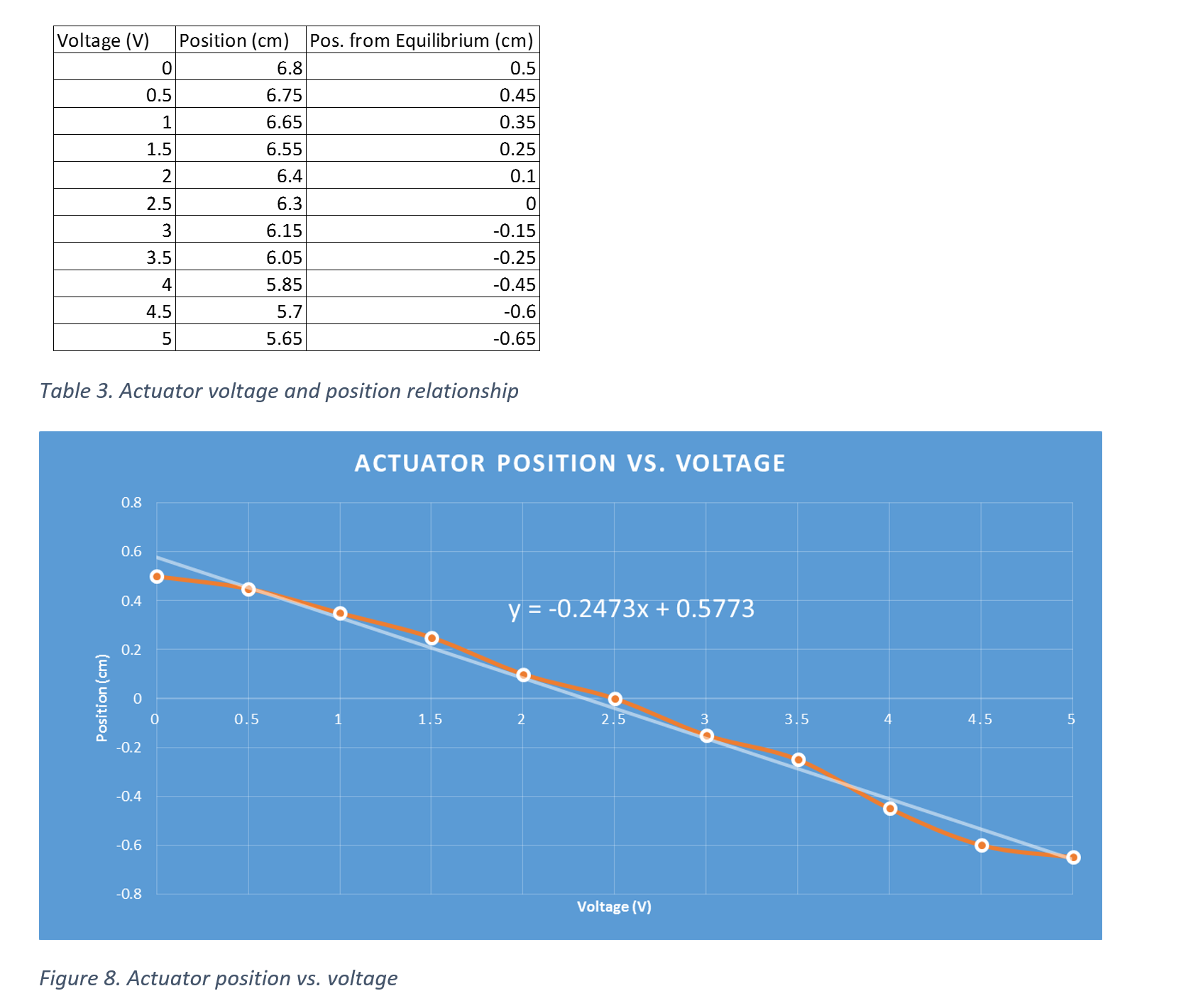
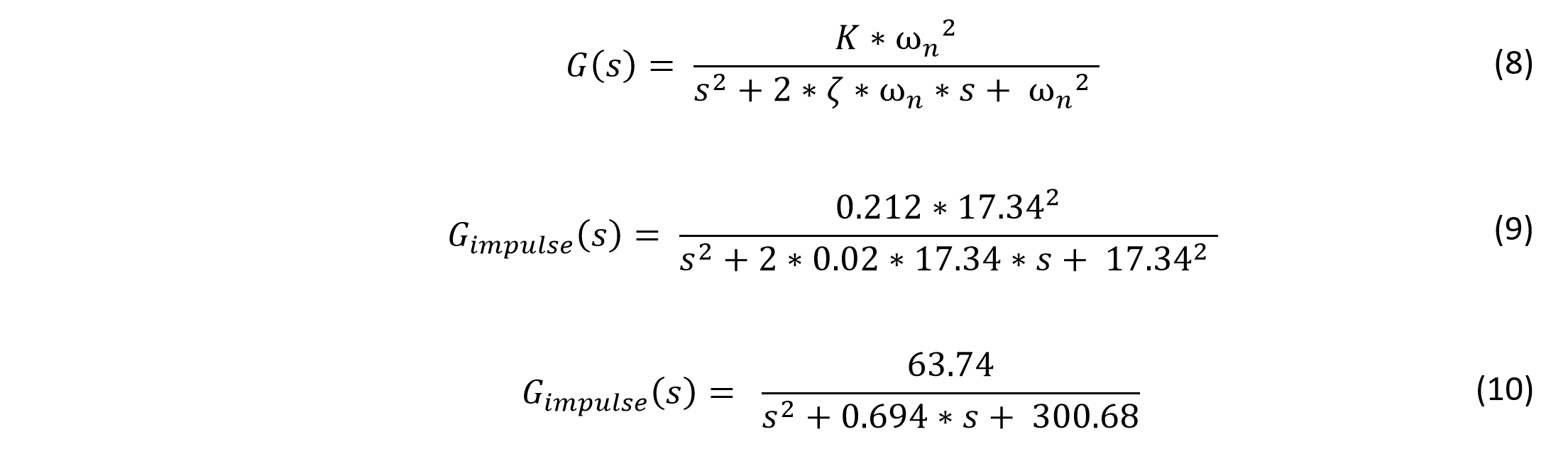
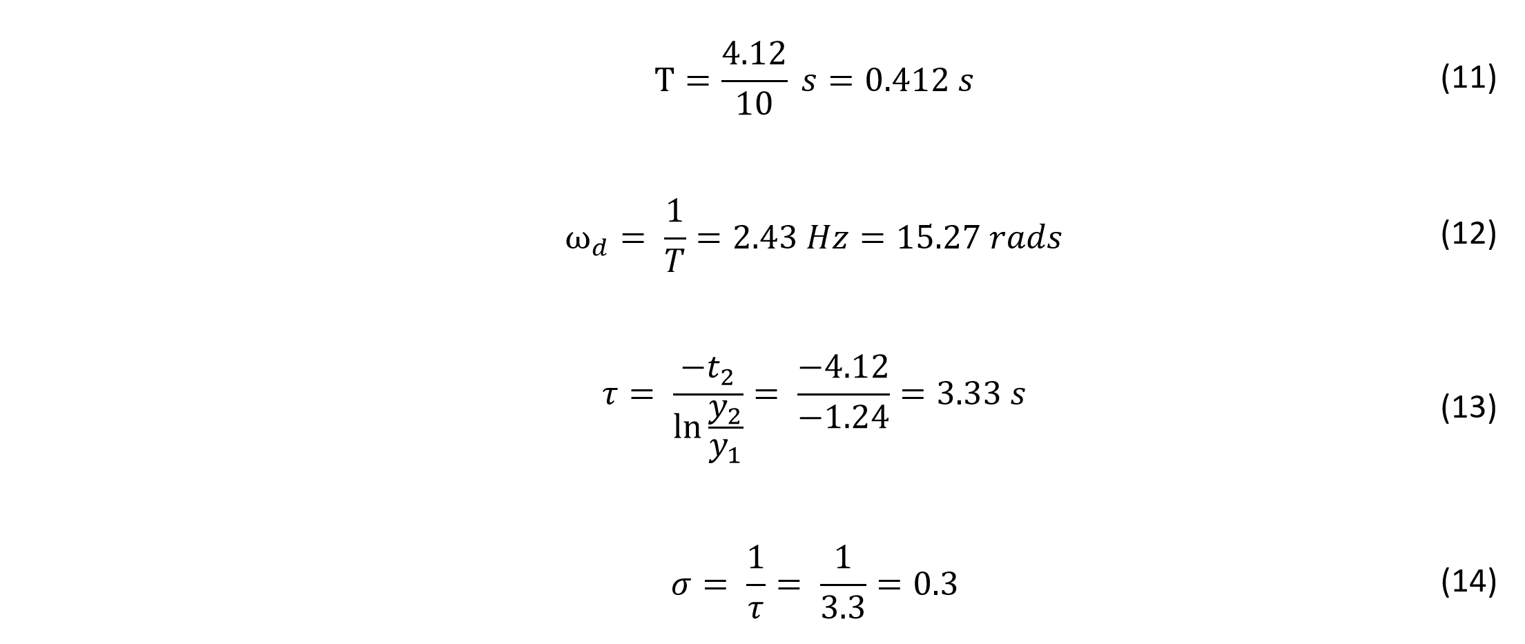
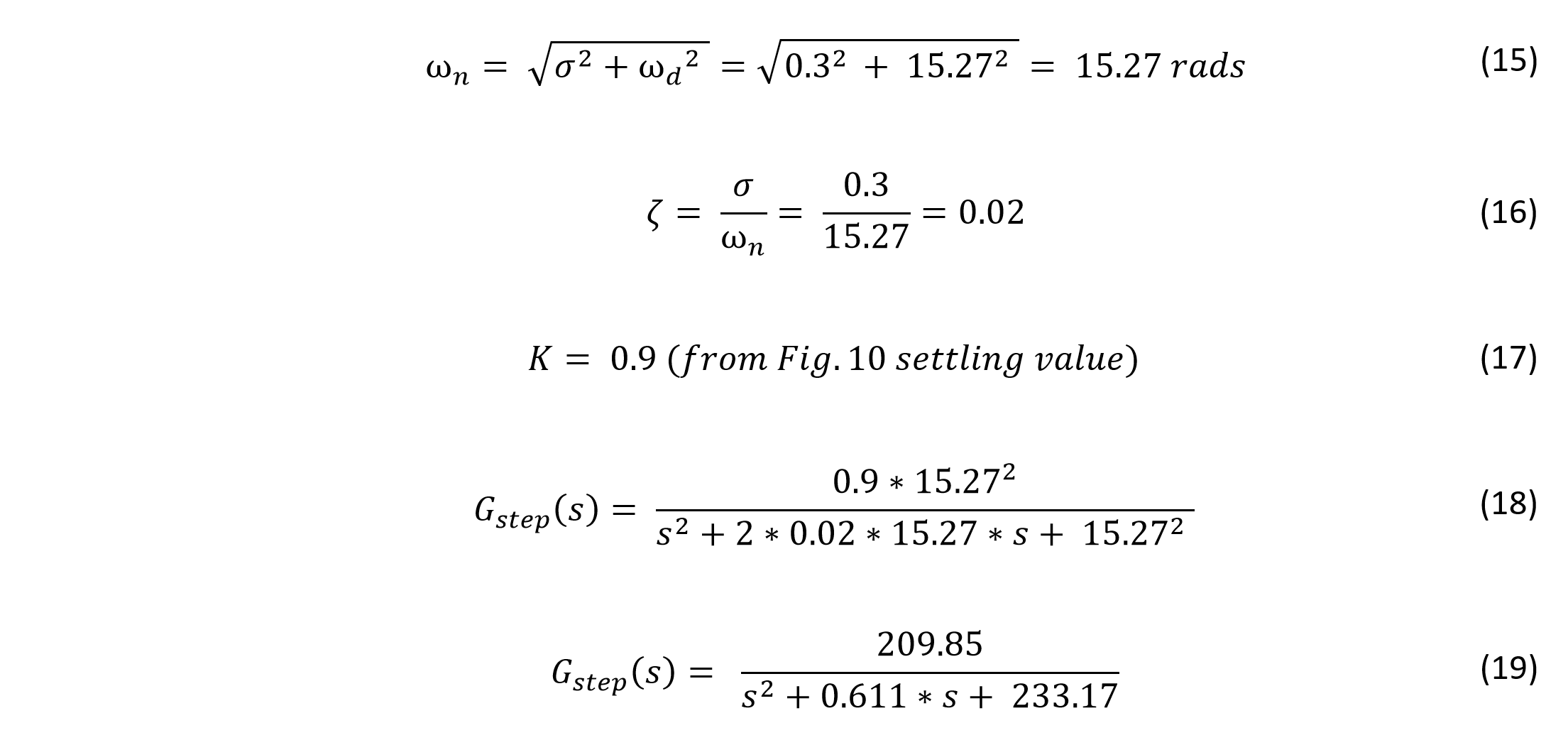
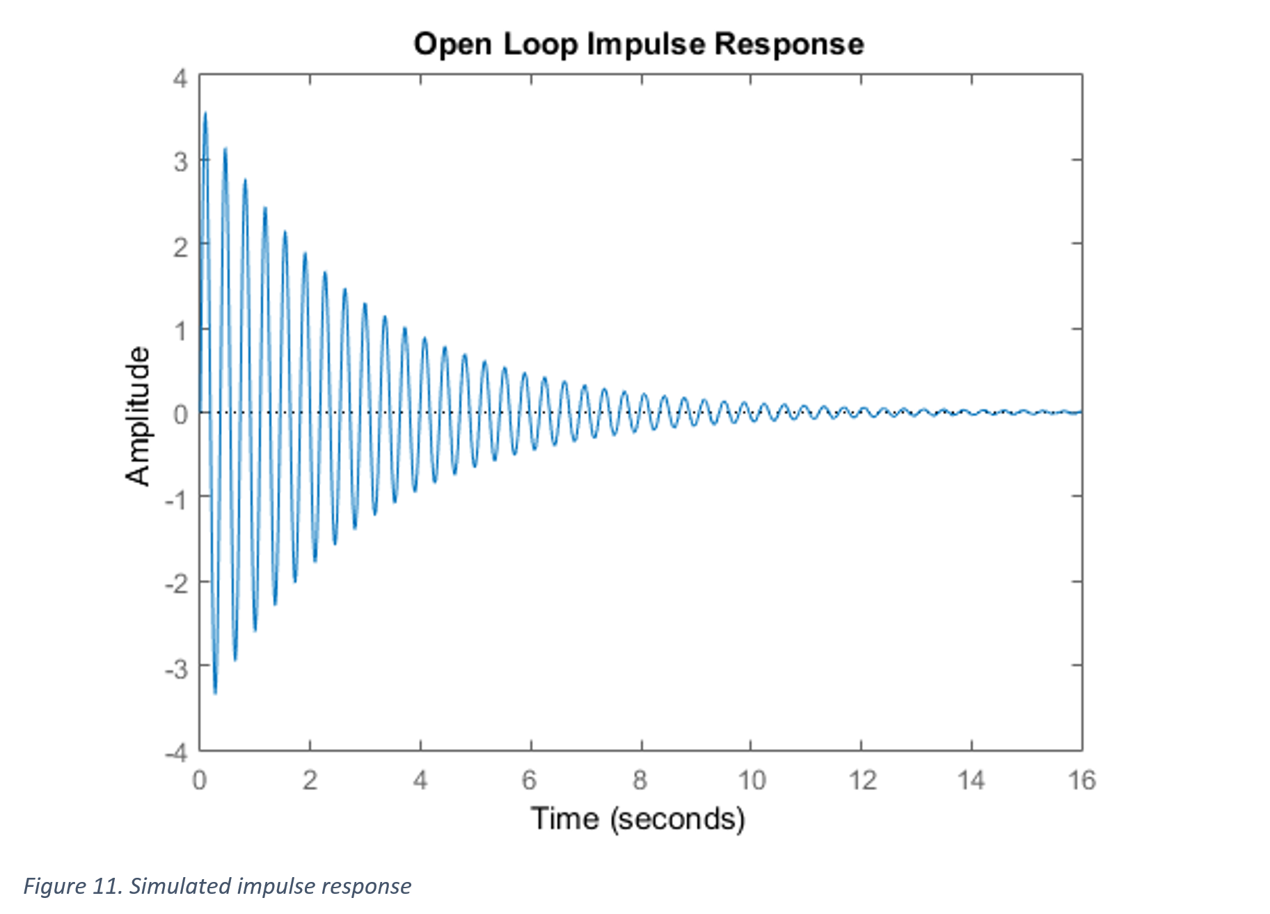
Previously, a continuous time domain transfer function for the teeter-totter was arrived at by means of impulse response.

To bring this continuous time s-domain transfer function into the z-domain, the z-transform must be applied.

This z-domain model now takes into account a sample time of 18 ms  and the zeroth-order hold to account for the data acquisition instruments.

Open Loop Control

Open loop control can be a desirable means of control for certain applications where disturbance rejection is not necessary. Additionally, open loop controllers can be applied in series with other methods of feedback control when it is desirable to reject disturbances to the plant. Open loop control is easy to implement and can allow a system to adjust to a reference point with little overshoot or steady state error, if any at all.

The following figure illustrates the implementation of an open loop controller F(z)

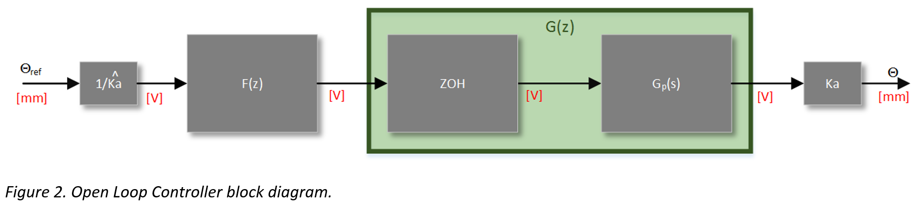
It can be seen that F(z) is a volt-to-volt transfer function, which explains the constant of 1/Ka  out front. This allows the input to the system to be a reference position. The inverse of the actuator gain is used rather than the sensor gain due to the nature of the open loop system. Because there is no feedback present, it would be nonsensical to use sensor gain. Note the hat above Ka designating the experimentally determined numerical value that is a model of the true behavior of Ka.

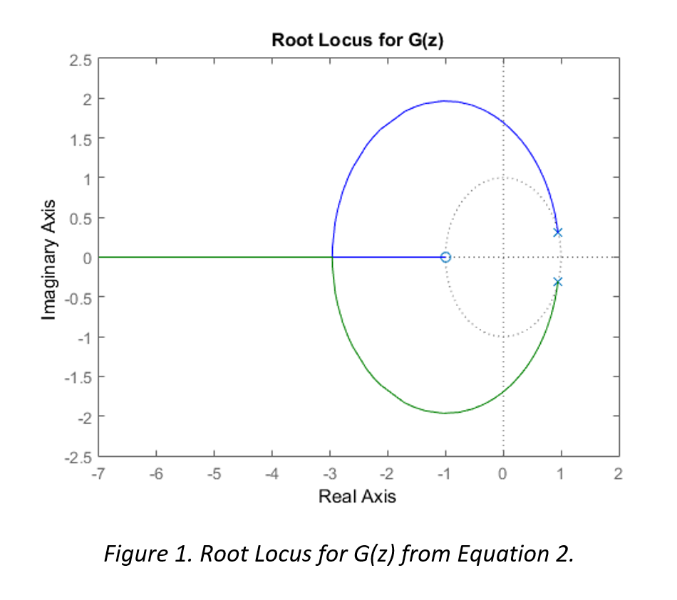
The implementation of an open loop controller is simple. The idea is to create a transfer function based on the current (undesired) pole locations of the plant transfer function G(z), and the desired pole locations. By placing the undesired (actual) G(z) pole locations in F(z)’s numerator, they will effectively “cancel” out the undesirable poles. With that being said, the poles will never truly cancel out even though they may appear to be canceling mathematically. Finally, F(z)’s denominator is set to be the desired pole locations.

F(z)’s denominator can be anything, but the idea is to force the system to behave in a desirable way. Ideally, the poles of G(z) would be repeated on the positive real axis, as close to the imaginary axis as possible. It is likely that this will not be achievable, as it will require more actuator energy than what is available. It is for this reason that a happy medium must be arrived at, where the desired behavior is in harmony with the system and its resources.

The following three figures illustrate the step response of the system FG(z) and the controller F(z)

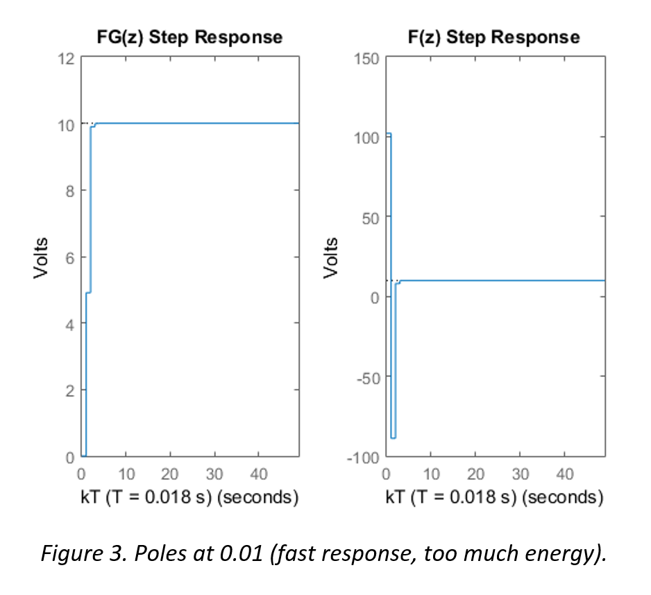
The simulation in Figure 3 shows the most ideal response characteristics, however, it would require an initial burst of over 100 V, which would exceed the limitations of the voltage supply and actuators.

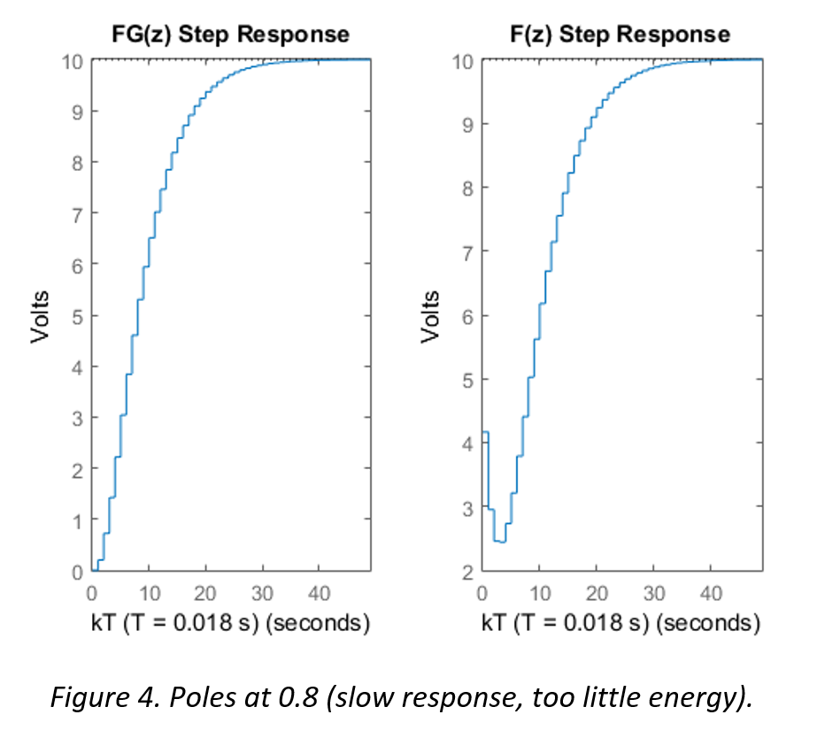
The simulation in Figure 4 shows a response which requires little energy, and it can be seen that the system takes a significantly longer amount of time to reach steady state when compared to the response time in Figure 3.

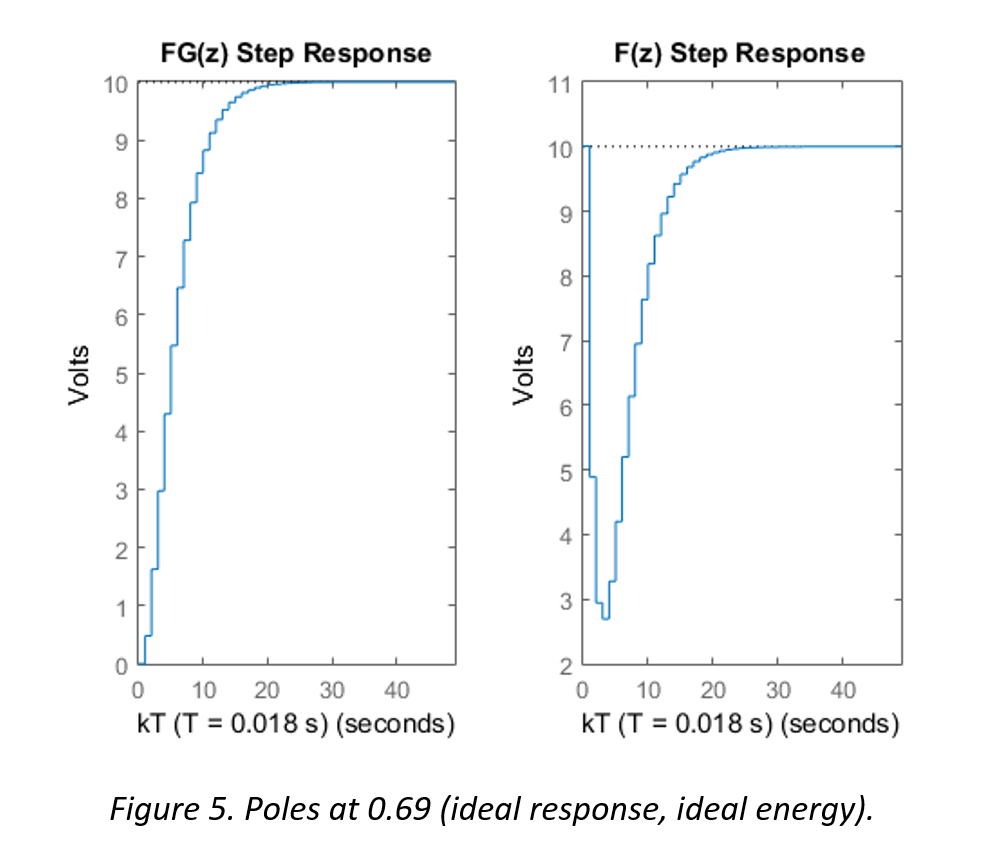
The simulation in Figure 5 shows the ideal balance between response time and energy requirements. The initial “push” does not exceed the limitations of the actuators or the supply, and the amount of time to settle at steady state is reasonable (approximately half of a second).

Therefore, the transfer function of F(z) is set to be

The actual outputs of FG(z) and G(z) can be seen in the following figure

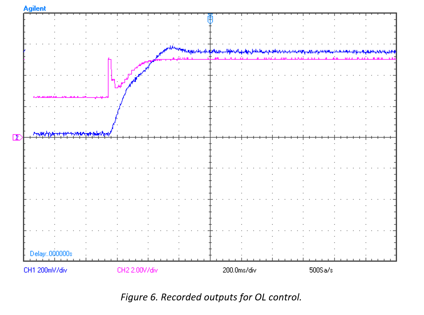
The pink line illustrates F(z)’s output, where it is coming from a DAC whose dynamic range is 0 to 5 volts. The blue line illustrates FG(z)’s output. Note the slight overshoot and settling time of approximately 0.5 seconds.

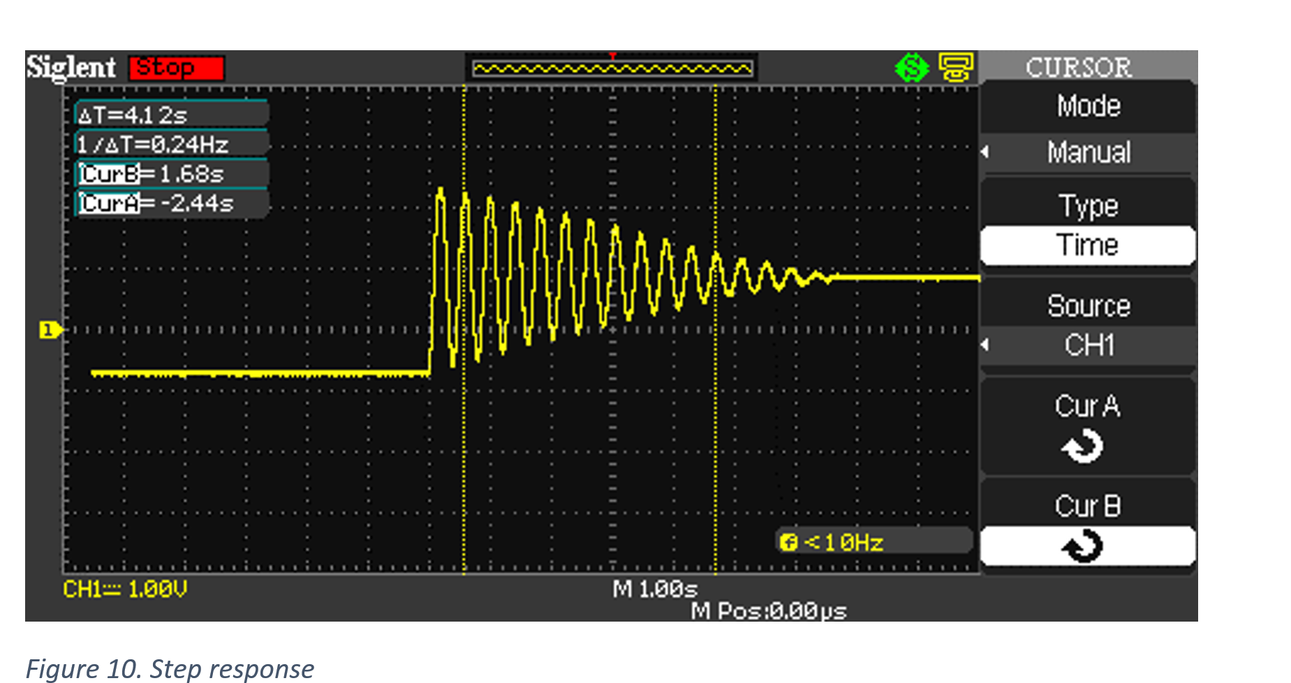
Uncompensated step response:

Compensated step response:

These GIFs demonstrate the reduction in settling time due to the open loop controller when the system is given the command to move to a new reference point.

Lead Compensation

Lead compensation is a type of compensation which improves the loop phase at the expense of the loop gain. Lead compensation is desirable in that it can be used to first stabilize the system with an acceptable phase margin before attempting to improve its performance. Lead compensators tend to speed up the transient response but will increase the steady state error. Additionally, lead compensation can increase system bandwidth and stability margins, and for this reason, is essential to systems that are unstable or on the border of instability.

The following figure illustrates the implementation of an lead compensator D(z)

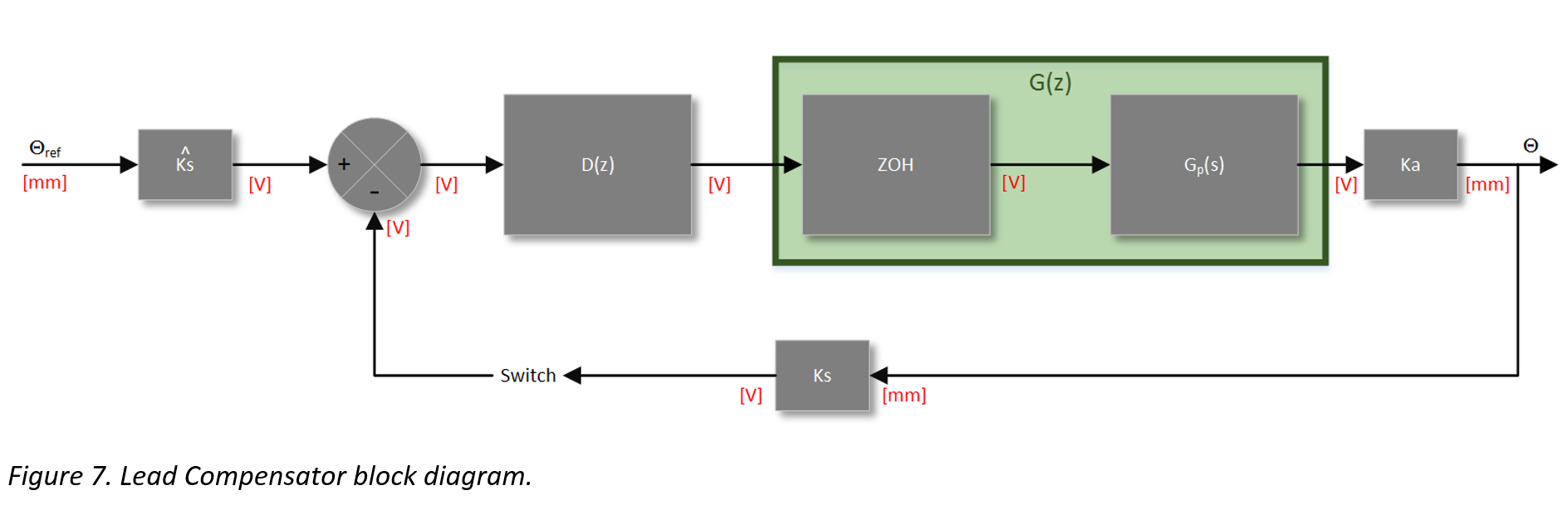
Because D(z) is a volt-to-volt transfer function, the Ks hat term must be applied to the input reference. The hat on Ks denotes that it is a model of the sensor gain, not the physical gain exhibited by the sensor which is found in the feedback loop.

The approach for implementing a lead compensator can be done in either the time or frequency domain. The idea is to satisfy the specifications on phase margin, gain crossover frequency, and steady state accuracy. To achieve this, a Bode plot of the plant is constructed and the phase curve is adjusted in such a way that the phase margin and gain crossover frequency requirements are met.

A phase lead compensator consists of a single pole and zero. Its transfer function can be described as

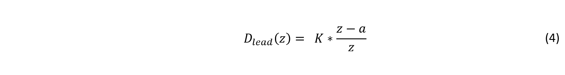
Where a pole exists at z = 0 and a zero exists such that a < 1.

In order to properly implement a phase lead compensator, the pole and zero must be placed in a manner that the benefits of the positive phase shift are achieved and the magnitude degradation is accounted for. The following figures illustrate the magnitude and phase frequency characteristics of a phase lead compensator D(z), the plant G(z), and the combined system DG(z).

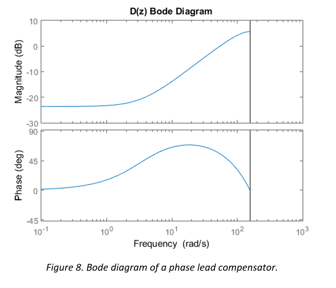
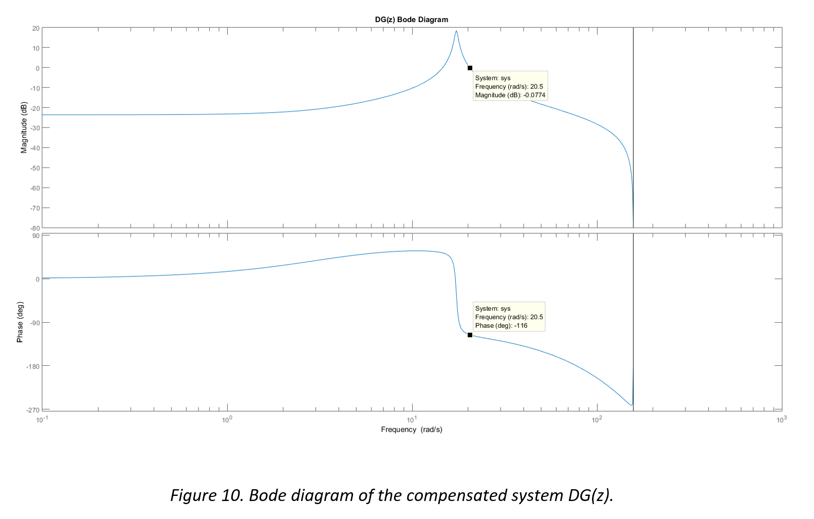
It can be seen in Figure 9 that the plant is unstable at the zero crossover frequency (the phase is less than -180°). Figure 8 illustrates a lead compensator which exhibits the phase lead required to stabilize the system, along with the undesirable but necessary degradation to the gain at lower frequencies. Figure 10 shows the combined result DG(z), where the system is now stable with approximately 65° of phase margin at the gain crossover frequency.

The transfer function for the lead compensator which resulted in these stability improvements is

The phase lead controller was implemented in a manner illustrated by Figure 7. The resulting controller and system outputs can be seen in the following figures.

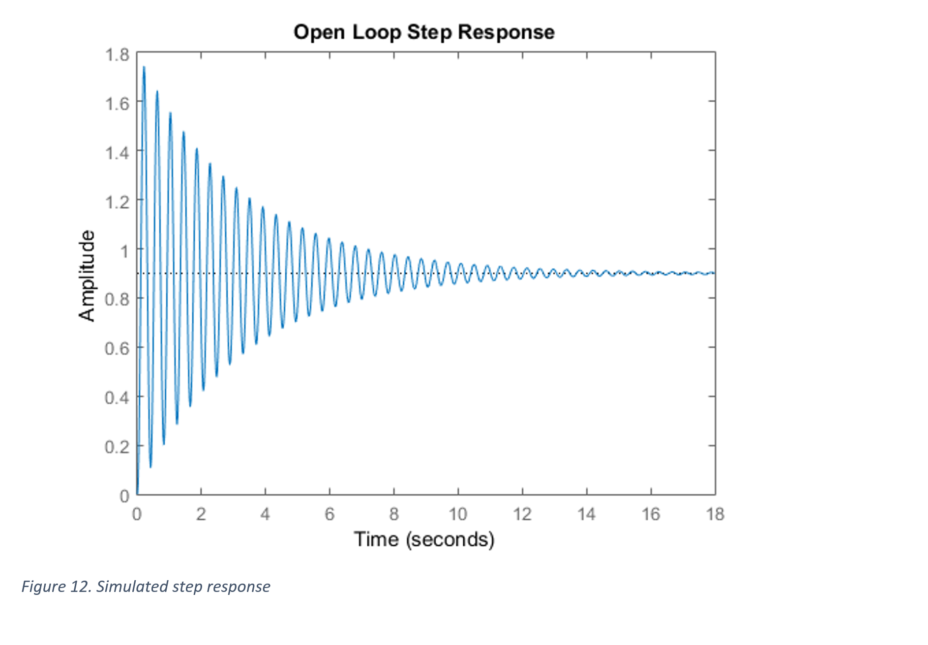
Note that the system now has the ability to be adjusted to a reference point with some undesired transient characteristics and steady state error (Figure 11), but can respond to impulse responses and reject disturbances (Figure 12).

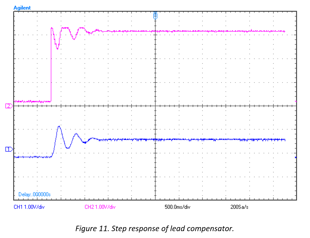
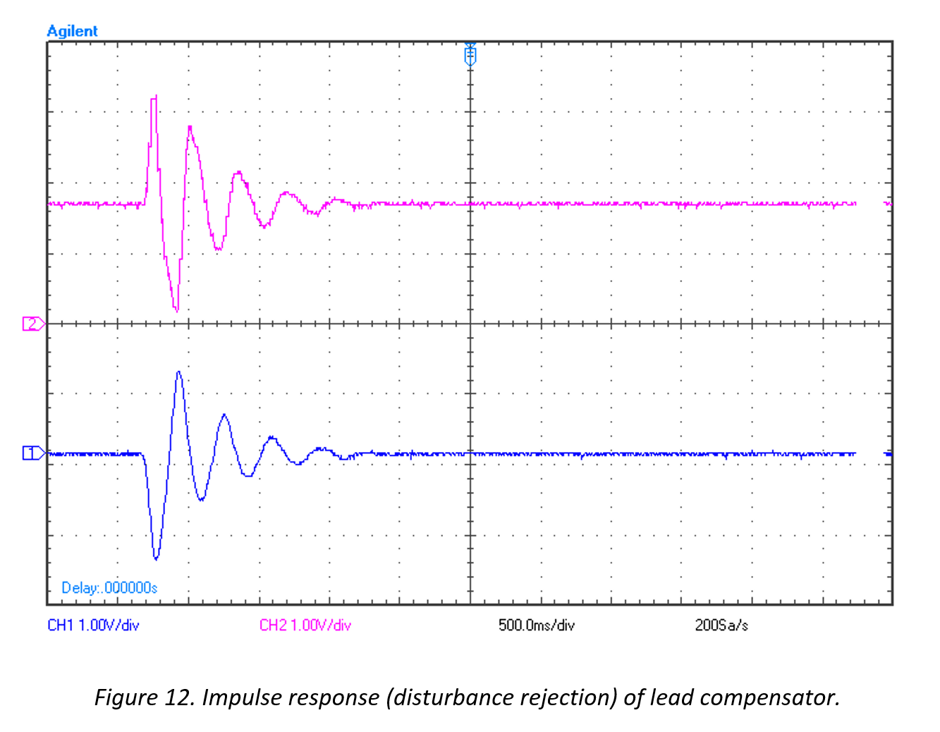
Note that the blue illustrates the system output and the pink illustrates the DAC output to the actuators.

Figure 12 shows a settling time improvement by a factor of 8. The system settles in approximately 1.5 seconds due to an impulse response, compared to the uncompensated system which settled in approximately 12 seconds.

Bridged-T Controller

The Bridged-T network is a style of compensation that utilizes the two previous methods of control in a way that harnesses the benefits of both methods. The idea is that the open loop controller will be used to “throw” the system to the desired location when a step response is seen at the input, and the lead compensator will take control only when there is an error signal present. In essence, the open loop controller does the heavy lifting and the lead compensator does the fine tuning once the system is in the ball-parked location. This style of control achieves better performance and accuracy than what could have been possibly using a traditional PID controller.

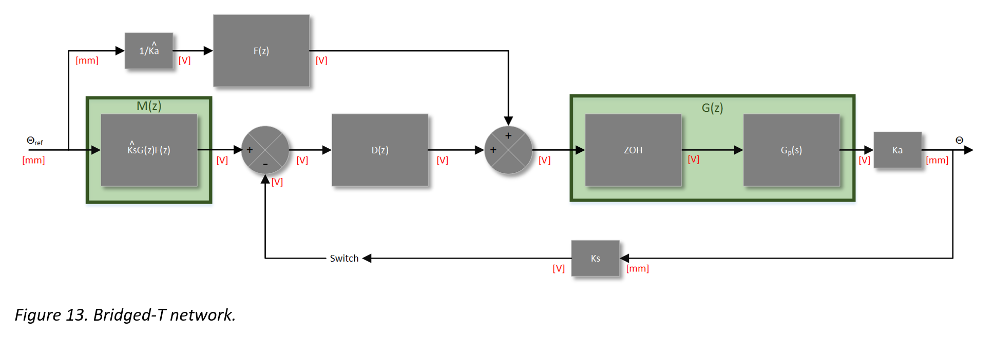
It can be seen in the diagram above that there are a few new elements introduced to the control scheme. There is a block M(z) and a feed forward path that contains the open loop controller. Additionally, there is a second summing junction after the lead compensator D(z). If there is no error signal present from the first summing junction, D(z) is effectively removed from the system (it has no effect), and the system will behave in a way such that its only form of control is coming from the open loop controller F(z).

If an error signal is present, it will be the result of the sensed position subtracted from (Ks)G(z)F(z). It is at this point in which the phase lead controller D(z) will correct any error in the system and provide disturbance rejection.

F(z) and D(z) are described by Equation 3 and Equation 5 respectively.

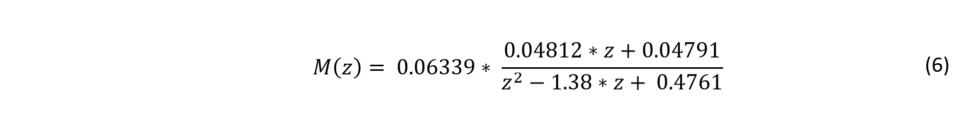
M(z) is described by the following transfer function

The following plots show the impulse and step response of the Bridged-T controlled system.

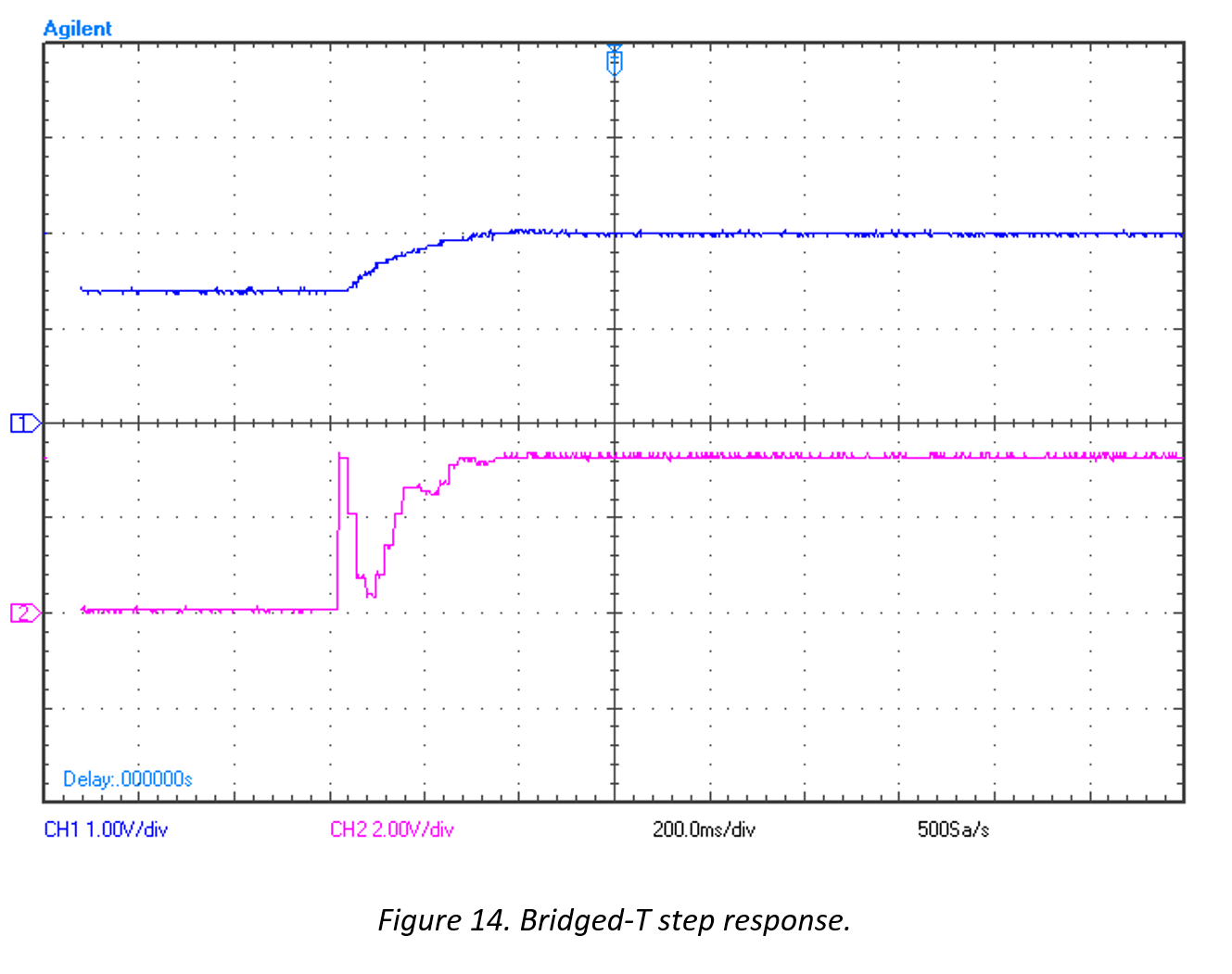
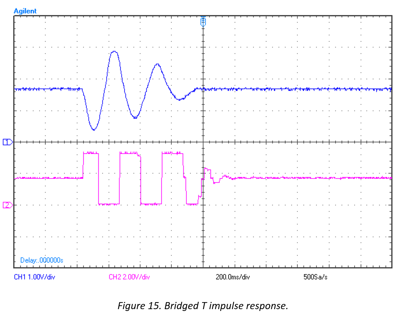
Note that the blue illustrates the system output and the pink illustrates the DAC output to the actuators.

Figure 14 shows improved transient and steady state error characteristics over the system which was previously controlled by only the lead compensator (Figure 11).

Figure 15 shows the system’s ability to still reject impulse disturbances. The system performs even better given (a settling time of approximately 600 ms, improvement factor of 20). This could be due to the fact that the control scheme was implemented in C code on an ARM Cortex M4 processor rather than with LabVIEW on the Agilent ADC/DAC tool.

Conclusion

After the teeter-totter was constructed, a model was derived by observation and applied to the prototypical second order system transfer function. This s-domain transfer function was brought into the z-domain by means of the z transform, only after the data acquisition characteristics had been corrected for by combining the zeroth order hold with the plant transfer function.

The first form of control that was examined was open loop control which provided the system with the ability to adjust to a reference point with little overshoot or steady state error, if any at all. The open loop controller was easy and quick to implement by examining where the undesired poles were located, “cancelling” them out, and introducing poles in locations that achieved the desired response.

The next form of control implemented was a form of feedback control known as phase lead compensation. The phase lead compensator consists of one pole and one zero such that the pole is less than the zero. Phase lead compensation was used not just to achieve stability, but to introduce a phase margin of nearly 65°. While the system was able to reject disturbances with a reasonable settling time, it lacked the DC gain and low steady state error of the open loop controller.

To get the best of both worlds, a “Bridged-T” compensator was implemented. This network combines the desired control effects exhibited by the two previous forms of control, one making up for what the other lacks. The open loop controller was used to “throw” the system to the desired location when a step response is seen at the input, and the lead compensator will take control only when there is an error signal present. In essence, the open loop controller was doing the heavy lifting and the lead compensator was fine tuning the system it was in the ball-parked location set by the open loop controller.

Out of my own curiosity, I implemented the Bridged-T controller in C code on an ARM Cortex-M4 to exercise the implementation of digital control systems on a microcontroller. The ARM Cortex-M4 proved to outperform the NI Data Acquisition tool. It decreased the settling by a factor of 20, up from the previous factor of 8 seen in the phase lead compensator.

This is part one of a two part series… check out the implementation of various control schemes in part two!

Buy me a coffee!

Abstract – A teeter totter will be constructed for the purpose of a sampled data control system demonstration. Upon completion of construction, the teeter totter and its sensor and actuator systems will be characterized to obtain a prototypical second order system transfer function. This model will then be used to design a controller and compensator for the system.

Construction 

For this exercise, the system will be a teeter totter. It is of interest to construct a system that exhibits as little amount of non-linearities as possible. The goal is to characterize its response and develop a control system that will decrease the teeter totter’s settling time by a factor of 10. The teeter totter will consist of four main parts:

1. A plane which is free to move about an axis with one degree of freedom
2. A post to hold the axle and elevate the plane
3. A base to secure the post and actuators
4. A system of sensors to allow for position information of the plane’s angle

The following images are of the 3D models that were created using Blender to generate parts 1, 2, and 3 by means of 3D printing.

The final constructed teeter totter can be seen in the following image with annotated points of interest:

The plane (1) has one degree of freedom of which it is free to rotate about the axis established by its axle (2). Skateboard ABEC-5 bearings are held in place by a hex bolt, two washers, and a nut. The bearings allow for a reduction of friction which will improve linearity. The axle post (3) attaches the plane and bearing assembly to the base (4). The permanent donut magnets (5, 6) are glued to a bolt which allows for fine elevation adjustments to be made. The sensor network is comprised of two infrared emitters (7) and a single infrared photo-diode (8). The sensor network was chosen to operate in the infrared spectrum so that the system would be impervious to ambient light. The actuator network is comprised of two electromagnets (9, 10) which operate together in an opposing fashion. Their magnetic fields will repel and attract the permanent magnets (5, 6) to actuate the plane.

The sensor network provides feedback to a controller which will then deliver control signals to the actuators. The infrared photo-diode will pass a current that is proportional to the amount of infrared light being received. This current is then converted to a voltage by passing it through a resistor to ground. The voltage is then correlated to the position of the plane.

The actuator network is wired in series. Its input comes from a push-pull network of complementary transistors. A current can be delivered to the base of the NPN/PNP transistor push-pull network by the controller, causing a current to flow in the desired direction through the coils in order to achieve the appropriate magnetic field orientation.

The following schematic describes the electrical setup of the sensors, actuators, ADC output and DAC input:

The connector (J3, J7) delivers power to the sensor network and converts the current to a voltage using an adjustable potentiometer. This voltage is then sent through a gain stage and an offset stage for conditioning to the ADC.

The actuator network (seen in Figure 5) works in a similar fashion, where the input form the DAC (J6) is conditioned by an offset stage and gain stage in order to deliver +/- 12V to the actuator coils.

A prototype was created which can be described by the previous schematics in Figures 4 and 5 (excluding voltage regulators) in addition to a printed circuit board.

Modeling

The sensor and actuator network was characterized in the following fashion: For the sensors, the plane of the teeter totter was manually positioned at various points and the corresponding output voltage was noted. For the actuators, an input voltage was delivered from -12 to +12 volts and the position of the teeter totter plane was noted. The results have been tabulated and can be seen in the following tables and plots.

From the results above, the data points have been characterized by the following linear equations

Sensors:

Actuators:

The absolute value of the slope from Equation 1 represents the sensor gain, Ks, and the absolute value of the slope from Equation 2 represents the actuator gain, Ka.

The system was then connected to an oscilloscope and power supply in order to obtain the impulse and step responses. The output voltages are obtained from the infrared sensors. They relate the position of the teeter totter’s plane to a voltage.

From Figure 9, twenty periods were used to find the average values of the period (T), damped frequency (ω­­­_d), natural frequency (ω_n), time constant (τ), damping coefficient (σ), and damping ratio (ζ).

The following calculations are with regard to the impulse response:

The transfer function can now be constructed from the obtained values. The prototypical transfer function for a second order system is

In a similar fashion, the transfer function can be obtained using the step response:

The transfer function obtained from the step and impulse response can now be plotted using Matlab:

Conclusion

The teeter totter constructed is suitable for a sampled data control system demonstration. While in its current state it still exhibits some nonlinear characteristics, it should be sufficient for moving forward to the next phase. The system can continue to be improved upon as a controller and compensator is being developed for it.

The next step is to develop a discrete model for what is currently a continuous time model. Once this is achieved, a microprocessor will be able to read in sensor data through an analog-to-digital converter, make control decisions based on the control scheme and sampled data, and output the appropriate control signals through a digital-to-analog converter.

This is part one of a two part series… check out the implementation of various control schemes in part two!