Analog filter design can be a tedious task, requiring frequency transformations, pages and pages of algebra, and many simulations to check that you are getting the response you designed for. Through the use of Geffe’s algorithm and Delyiannis-Friend circuits, bandpass filter design can be partially automated.
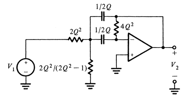
Delyiannis-Friend circuit with unity gain [1]:
The purpose of this post isn’t to detail the specifics behind Geffe’s algorithm, but rather to share with you a python script I wrote that will apply Geffe’s algorithm to a given set of input parameters, and output the required component values for each Friend circuit.
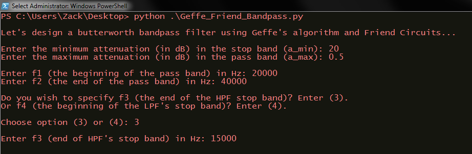
It is required that you have Python3 along with numpy, matplotlib, and scipy installed on your machine. The script can be executed through the Powershell if you are a Windows user by navigating to the directory where the Geffe_Friend_Bandpass.py file is located and then typing: python .\Geffe_Friend_Bandpass.py
Upon execution, the python script will prompt you for some input parameters.
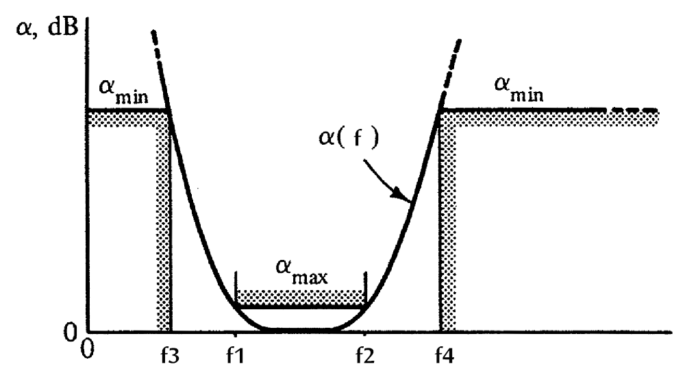
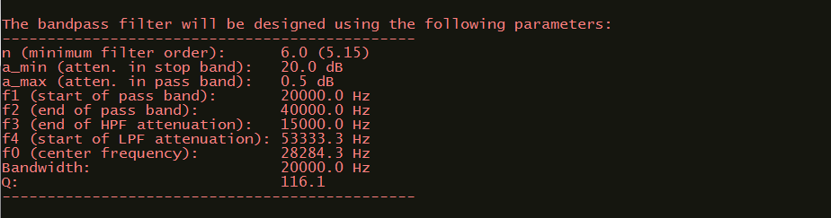
You are first asked for the maximum attenuation in the stop bands and the minimum attenuation in the pass band.
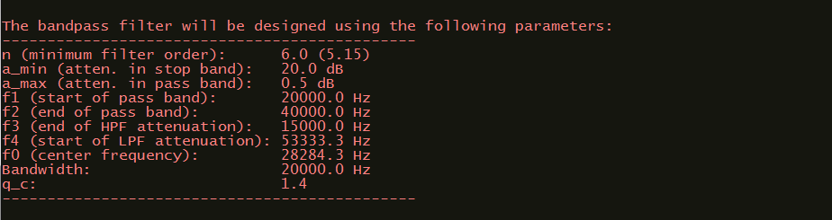
Then, you are asked to specify the pass band frequencies (f1 and f2) and one of the stop band frequencies (f3 or f4). The other stop band frequency is solved for automatically. See the following image [1]:
Parameter Details
The script will then return to you the information you had just entered, along with the minimum order filter required to meet your specifications.
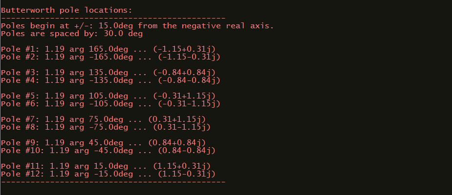
Butterworth Pole Locations
The locations of the poles are returned in both polar and rectangular format.
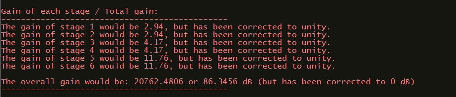
Gain Information
The gain of each stage is normalized to unity, resulting in unity gain at the center frequency.
The script can be tweaked to create a filter/amplifier, or an additional amplifier can be added after the filter.
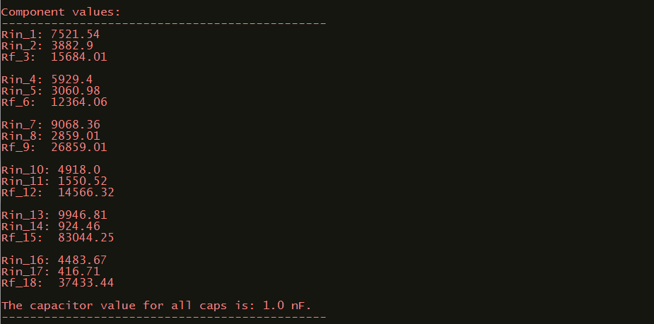
Required Resistor and Capacitor Values
The script will automatically calculate reasonable component values for each Friend circuit.
Note that n operational amplifiers (Friend circuits) are required for an nth order filter.
Click on the image to enlarge it, notice how the resistors and capacitors correspond to the output generated by the python script.
This example can be used as a general case, and the same arrangement will arise for any nth order output.
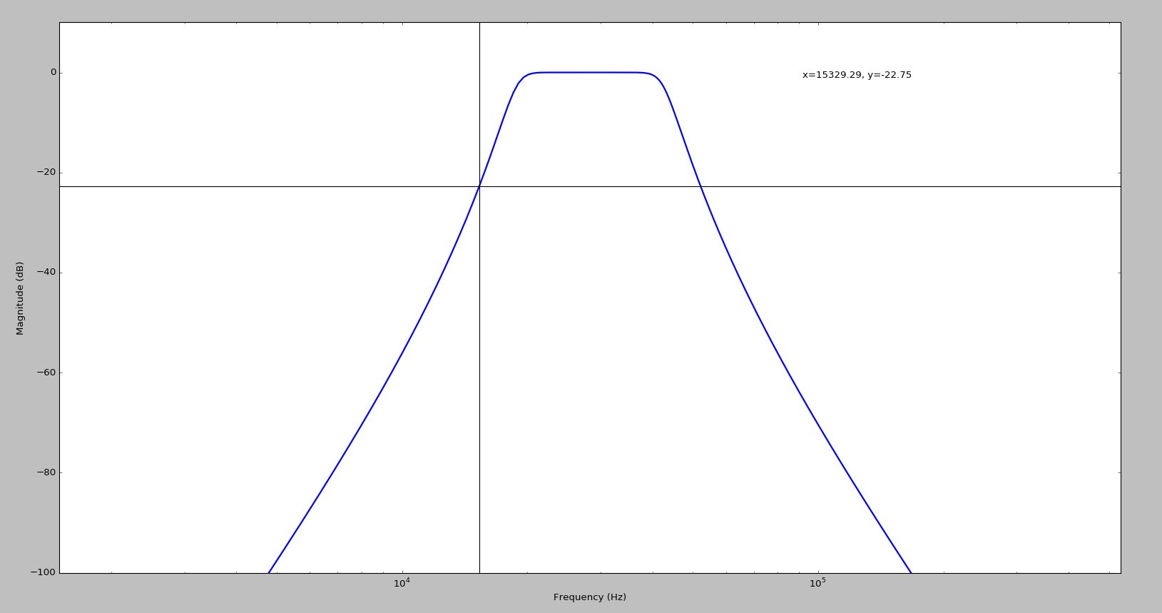
Auto Generated Bode Magnitude Plot
The script will then call on matplotlib to generate the bode magnitude plot of the filter. Interactive cursors have been added to allow for inspection of the pass and stop band frequencies.
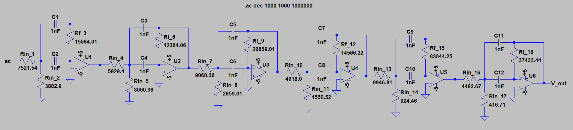
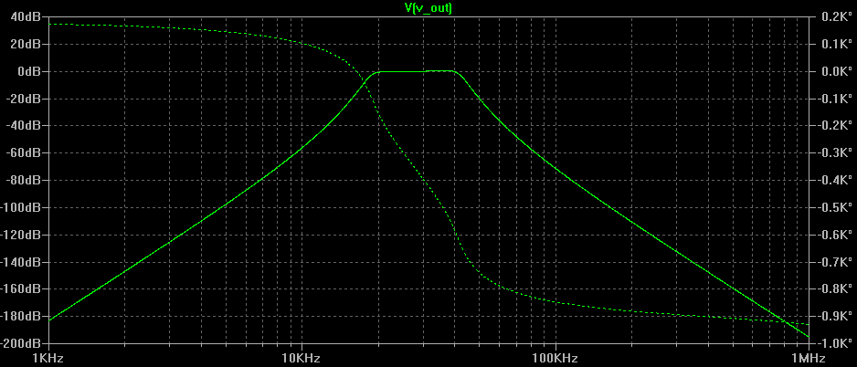
Plotting in LT Spice (AC Sweep)
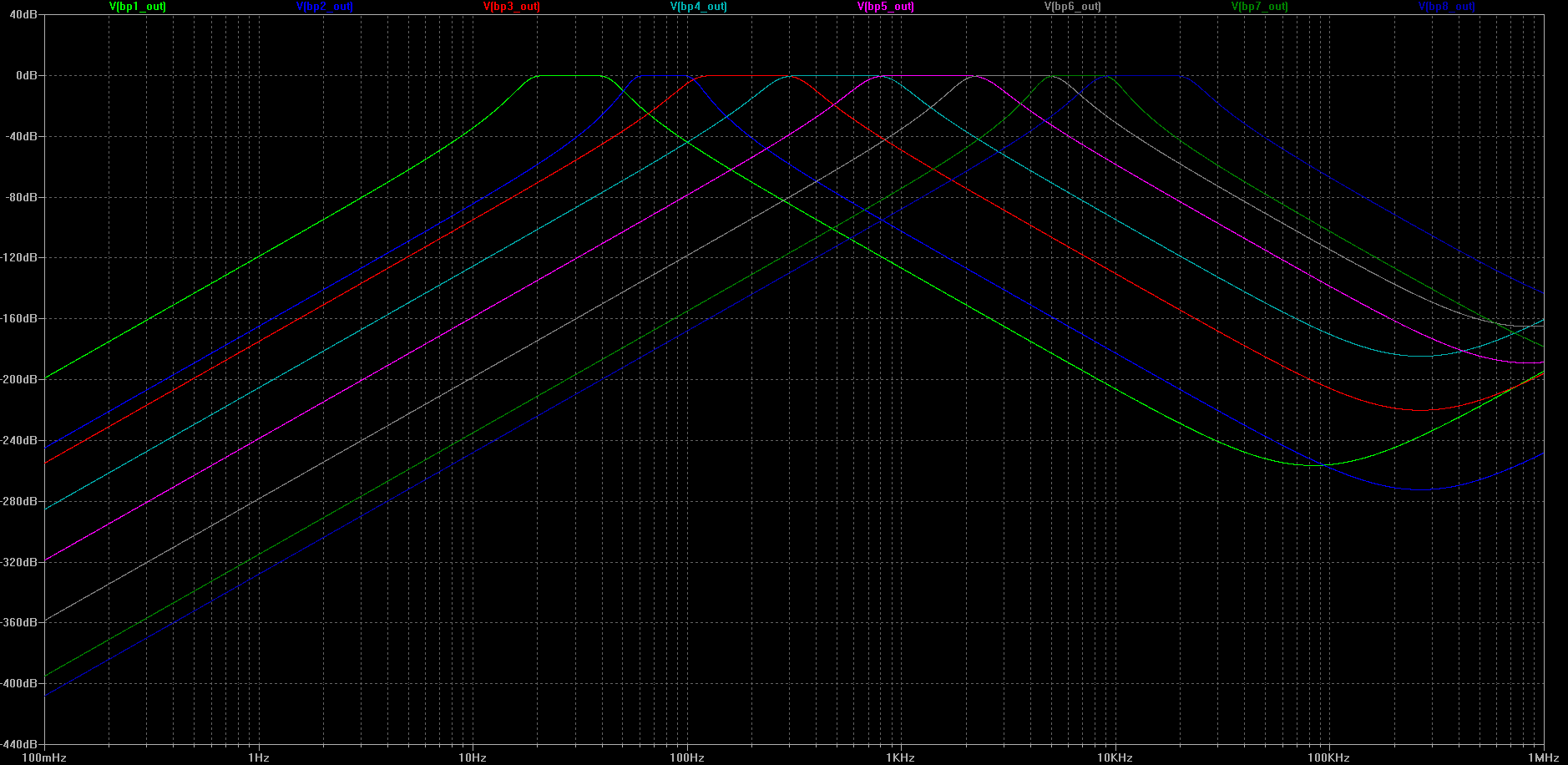
Here is the frequency response of the circuit once it had been built in LTSpice:
Conclusion
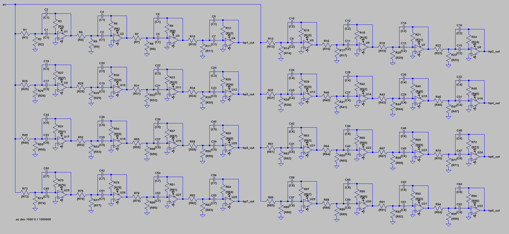
So what is this script good for? Let’s say you wanted to build a circuit that required multiple analog bandpass filters, but don’t want to crank out all the math to calculate the component values.
you would need 8-10 bandpass filters to select for various bands of the audio spectrum. You could use this script to design 8 bandpass filters very quickly!
Analyzing continuous signals by means of discrete methods requires special considerations in order for the results to be meaningful and accurate. Underlying this task is an exercise of optimization, where the capturing of continuous information must be in harmony with the constraints of the digital system. The goal is to spend the least amount of computational resources required to digitally represent a continuous signal.
Throughout this exercise, theory and principles that have arisen out of a half of a century of communication systems and signal processing study will be defined, applied, and demonstrated by example through computational software.
These principles include:
Bridging the analog and digital domain using the Nyquist-Shannon sampling theorem.
Representation of discrete signals in time and frequency domain using the Fast Fourier Transform algorithm.
Defining essential bandwidth using Parseval’s theorem.
Detecting energy signals by means of autocorrelation and ESD comparison (Fourier pairs).
It will be necessary to examine signals with domains in both time and frequency, as each domain gives access to different information contained within the signal.
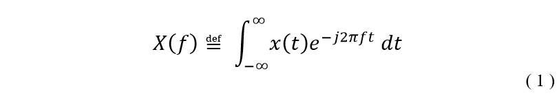
The Fourier Transform is a technique for mapping a function between its time/frequency or space/wavenumber domains.
The Fourier Transform is defined as follows
In everyday human experience, the signals we perceive are essentially continuous. For example, the sound waves produced by an Opera singer or heat transfer between two objects are processes which can take on an infinite number of values and exist continuously in time. This is in opposition to discrete signals which exist as packets that can take on a finite number of values and are discontinuous.
With the advent of digital computation, scientists and engineers now have the ability to solve complex problems where closed form solutions do not exist or are too difficult to obtain. In order for a digital computer to perform computations on such problems, they must be done numerically rather than analytically. For this reason, a signal that is continuous must be broken down into discrete components in such a way that its essence is captured.
Sampling, as stated previously, is the process of breaking down a continuous signal into a numeric sequence. The Nyquist-Shannon sampling theorem states that [1]:
If a function x(t) contains no frequencies higher than cps (counts per second), it is completely determined by giving its ordinates at a series of points spaced 1/2B seconds apart.
A sufficient sample-rate is therefore 2B samples/second, or anything larger. Conversely, for a given sample rate (fs) the band limit for perfect reconstruction is B ≤ fs/2.
Oftentimes, it is only necessary to consider a certain range of frequencies within a signal. While a signal may theoretically have infinite bandwidth, nearly all of its energy is likely be contained within a finite bandwidth of frequencies – this frequency range is known as the essential bandwidth of a signal. To define the essential bandwidth of a signal, Parsevel’s theorem can be used to evaluate the amount of energy contained within a bound of frequencies [2].
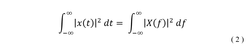
Parseval’s theorem can be expressed as follows
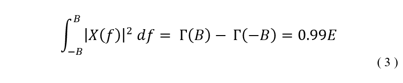
What this implies is that the total energy contained within a time domain waveform summed across all time is equal to the total energy contained within that same signal’s frequency domain waveform summed across all frequencies. From this, an arbitrary variable B can be assigned to the bounds of the infinite sum and set equal to a percentage of the total energy of the signal. Using the fundamental theorem of calculus, a closed form solution can be found. Consider the following example where
The variable B can be solved for provided that the total energy E is known and |X(f)|2 is integrable. Solving for B in the example above would provide the bandwidth necessary to capture 99% of the signal’s total energy. Alternatively, the essential bandwidth can also be solved for numerically by an iterative process.
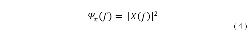
Because signals can exist in one of two forms, power or energy, it may be of interest to establish the form of a given signal. It is known that for an energy signal, its energy spectral density (ESD) and autocorrelation functions form a Fourier pair. The ESD of a signal is defined as follows
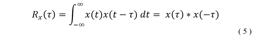
And the autocorrelation of a signal is defined as follows
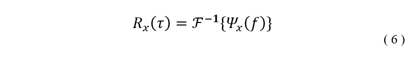
If the signal x(t) is an energy signal, the resulting Fourier pair exists such that
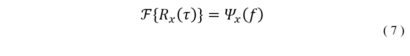
And vice-versa
Discretization of Continuous Signals
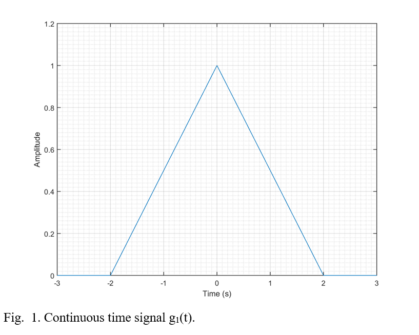
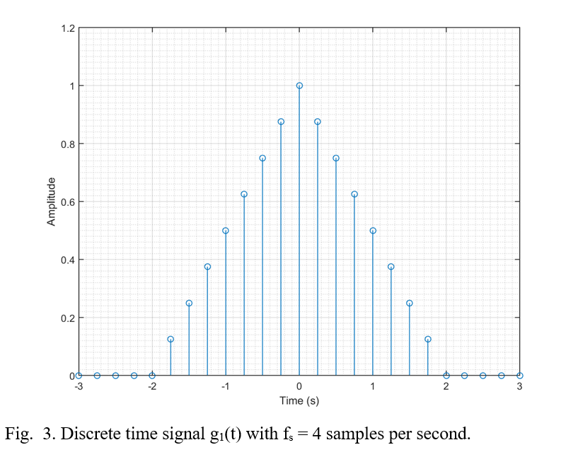
Consider the signal g1(t) = Δ(t/2) . This signal is defined for all values of time.
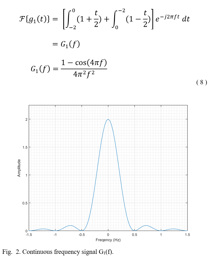
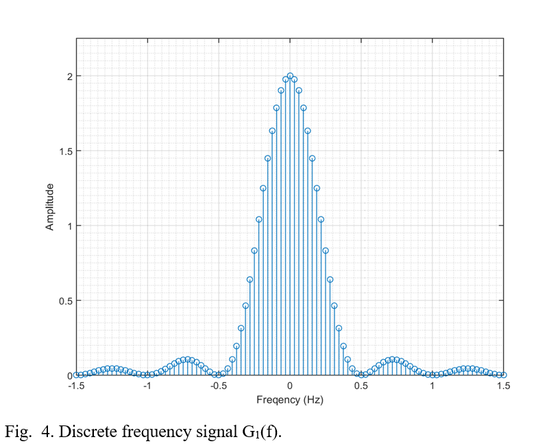
To determine the necessary sampling rate for this signal, its essential bandwidth must be established. By taking the Fourier transform of this signal, the magnitude of its frequency components will become apparent.
It can be seen in Fig. 2 that the signal’s magnitude is significantly reduced at frequencies greater than 0.5 hertz and less than -0.5 hertz.
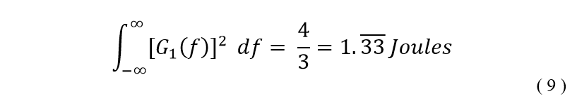
To determine this signal’s essential bandwidth, the signal’s total energy must be must be found for all frequencies.
The total energy of this signal can be found by integrating the square of the frequency components over all frequencies. From Equations (3) and (8)
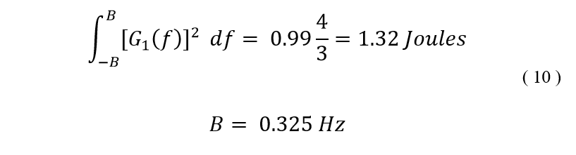
It is desired to capture 99% of this signal’s energy, so by assigning a variable to the limits of integration and setting the integral equal to 0.99 times the total energy, the essential bandwidth can be found.
From this result, the Nyquist-Shannon sampling theorem suggests that a sampling frequency as low as 0.65 samples per second can be used. Because this frequency is extremely low relative to the number of instructions a modern processor can handle per second, a modest sampling frequency of 4 samples per second will be used for the following simulations.
The discrete versions of this signal at a sample rate of four samples per second can be seen in Fig. 3 and Fig. 4.
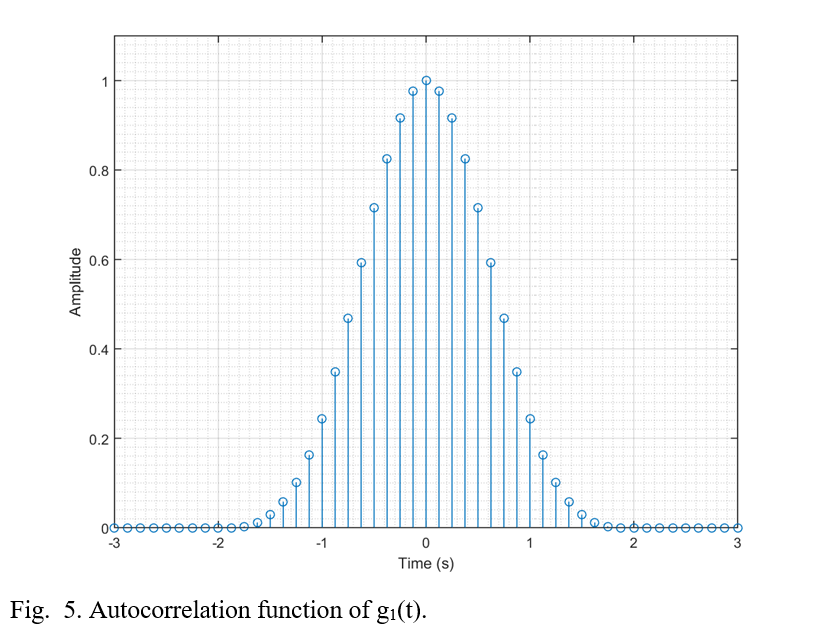
The autocorrelation function compares a time domain signal with a shifted version of itself. The resulting function is defined in Equation (5).
Performing autocorrelation on the discrete signal g1(t) results in the following time domain waveform
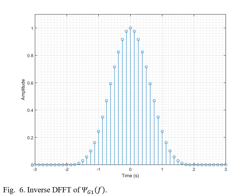
Given that g1(t) is an energy signal, the same discrete waveform should result from taking the inverse FFT of its ESD function. The ESD function is defined in Equation (4).
Performing the inverse FFT on ψg1(f) results in the following time domain waveform
It can be seen in Fig. 5 and Fig. 6 that g1’s autocorrelation function Rg1(τ) and ESD function ψg1(f) are indeed Fourier pairs.
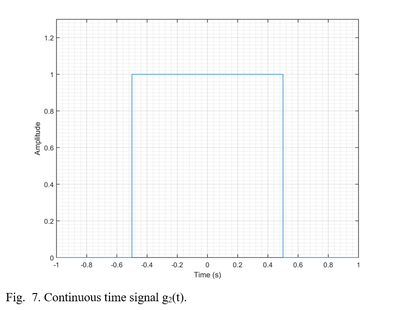
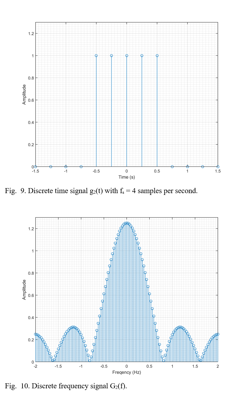
Next, consider the signal g2(t) = ∏(t) . This signal is defined for all values of time.
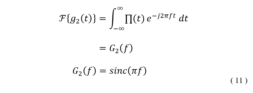
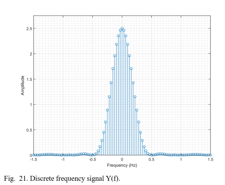
Like in the previous example, performing a Fourier transform on this signal will reveal the magnitudes of the frequency components across all frequencies.
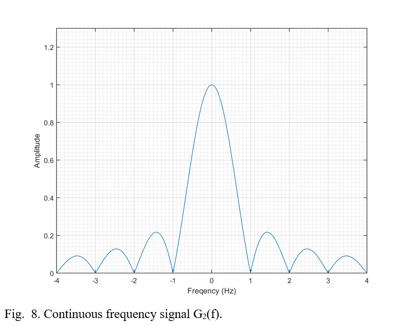
It can be seen in Fig. 8 that the magnitude of G2(f)’s frequency components do not diminish as quickly as G1(f) did.
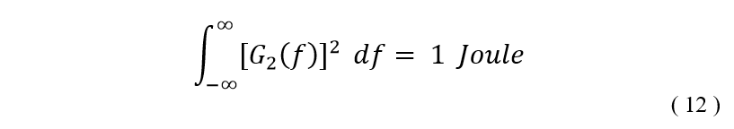
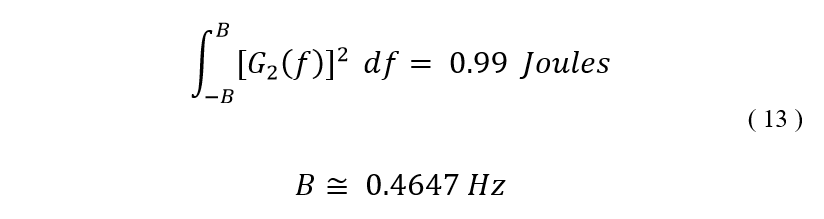
To find the total energy of this signal, the square of the frequency components are integrated over all frequencies. From Equations (3) and (11)
It is desired to capture 99% of this signal’s energy, so by assigning a variable to the limits of integration and setting the integral equal to 0.99 times the total energy, the essential bandwidth can be found.
To stay consistent with the previous signal g1(t), a sampling frequency of 4 samples per second will also be used for g2(t), as it exceeds the fs ≥ 2B rule established by the Nyquist-Shannon sampling theorem. The discrete versions of this signal can be seen in Fig. 9 and Fig. 10.
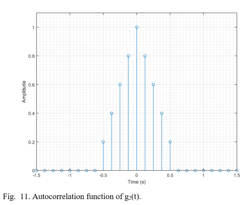
Performing autocorrelation on the discrete signal g2(t) results in the following time domain waveform
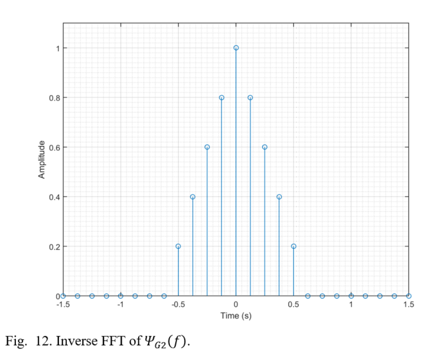
Performing the inverse FFT on ψG2(f) results in the following time domain waveform
Because g2(t) is also an energy signal, the autocorrelation function Rg2(τ) and ψG2(f) are Fourier pairs, as illustrated by Fig. 11 and Fig. 12.
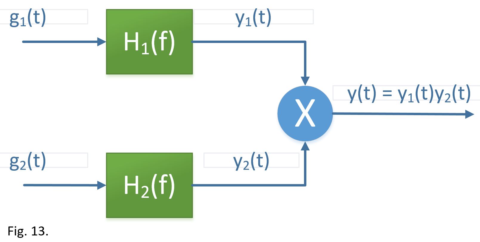
Now, let us consider the system shown in Fig. 13.
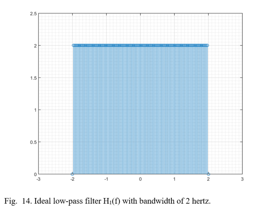
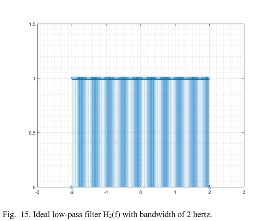
The blocks labeled H1(f) and H2(f) are ideal low pass filters with a bandwidth of 2 hertz.
The discrete frequency representation of the filters can be seen in the following figures
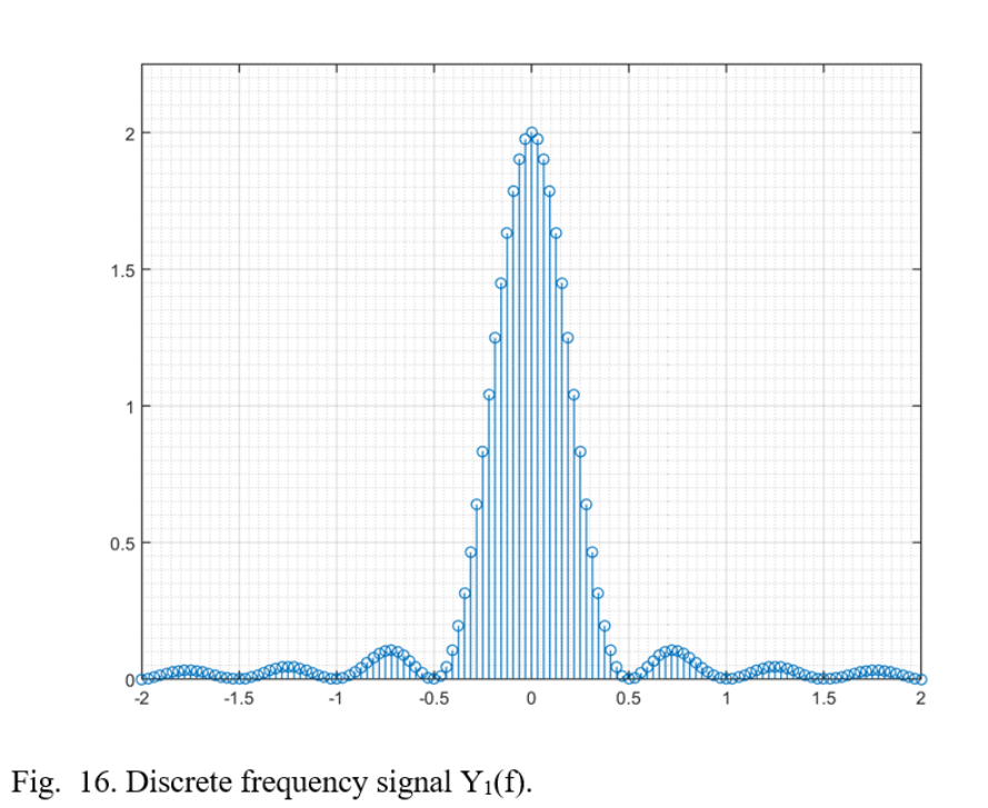
Passing the signal G1(f) through the ideal LPF H1(f) results in the following discrete waveform
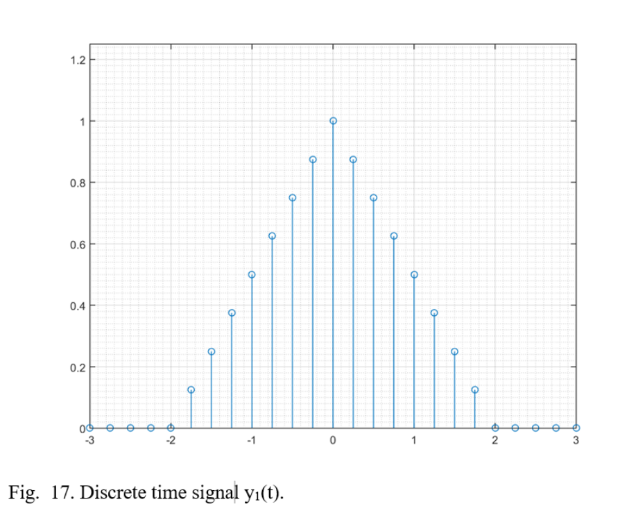
Performing an inverse FFT on the signal Y1(f) = G1(f)H1(f) results in the following signal y1(t)
Reconstructed in this fashion, it can be seen that the signals g1(t) [Fig. 3] and y1(t) [Fig. 17] are remarkably similar even with all frequency components greater than/less than 2 hertz removed from y1(t).
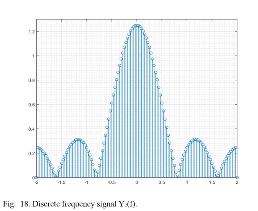
Passing the signal G2(f) through the ideal LPF H2(f) results in the following discrete waveform
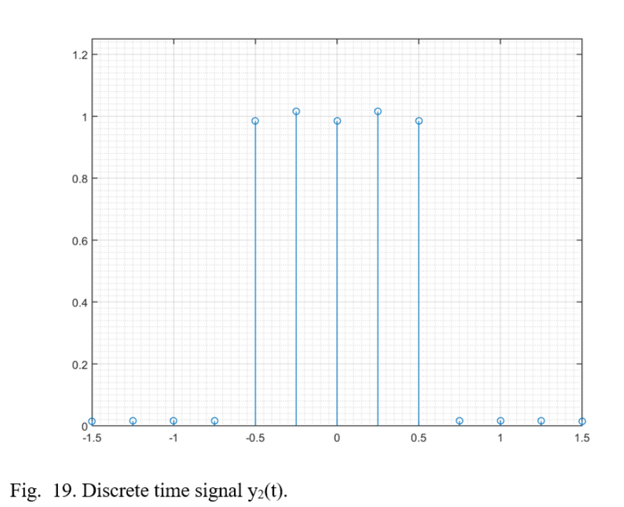
Performing an inverse FFT on the signal Y2(f) = G2(f)H2(f) results in the following signal y2(t)
Unlike the previous example with g1(t) and y1(t), it is evident that there are some imperfections resulting from the reconstruction of y2(t). This could be due to the fact that the ideal low-pass filter with a bandwidth of 2 hertz was not able to capture the signal in its entirety. Signals that exhibit abrupt changes in time, such as the changes that occur around the corners of the rectangular function, require higher frequency (energy) components. Filtering out these components will produce smoother and more oscillatory like behaviors in such areas.
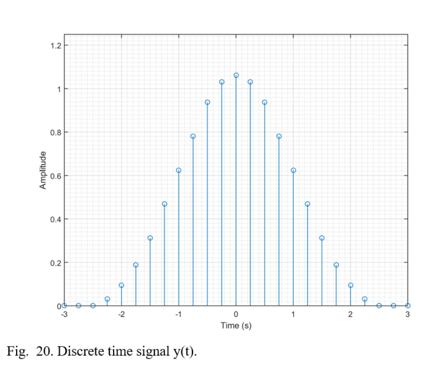
Mixing y1(t) with y2(t) results in the signal y(t). The following figures illustrate both time and frequency domains of the final signal
Conclusion
In order to effectively process continuous signals on a digital system, the signal bandwidth must be known. By applying the Nyquist-Shannon sampling theorem and Parseval’s theorem, the essential bandwidth of a signal can be defined and a sampling rate can be chosen. Choosing a sample rate that is too high will unnecessarily increase the demands on the processor and amount of memory required, while choosing a sample rate too low will result in loss of information and aliasing.
It should be noted to the reader that the FFT function contained within the MATLAB software requires special attention when attempting to properly scale in both time and frequency.
When performing an FFT, it is necessary to first perform an FFT Shift with the FFT of the desired signal inside its argument. For example
G1 = fftshift(fft(g1));
When attempting to plot a function in the frequency domain that resulted from a time domain function, such as the one above, the magnitude of the signal must be scaled down by a factor of the sampling frequency. For example
fs_g2 = 4; %sampling frequency for g2
normalize_g2 = fs_g2; %normalizing factor
G2_scaled = (G2)/normalize_g2; %divide G2 by normalizing factor
References
[1] “Communication in the presence of noise”, Proc. Institute of Radio Engineers, vol. 37, no. 1, pp. 10–21, Jan. 1949.
[2] Parseval des Chênes, Marc-Antoine “Mémoire sur les séries et sur l’intégration complète d’une équation aux différences partielles linéaire du second ordre, à coefficients constants” presented before the Académie des Sciences (Paris) on 5 April 1799.